Expressions

A guide for the defining and understanding the variable expressions used in InfiniteOpt. See the technical manual for more details.

Overview

Expressions in InfiniteOpt (also called functions) refer to mathematical statements involving variables and numbers. Thus, these comprise the mathematical expressions used that are used in measures, objectives, and constraints. Programmatically, InfiniteOpt simply extends JuMP expression types and methods principally pertaining to affine and quadratic mathematical expressions. A natively supported abstraction for general nonlinear expressions is planned for development since that of JuMP is not readily extendable.

Parameter Functions

As described further below, InfiniteOpt.jl only supports affine and quadratic expressions in its current rendition. However, there several use cases where we might want to provide a more complex known function of infinite parameter(s) (e.g., nonlinear setpoint tracking). Thus, we provide parameter function objects that given a particular realization of infinite parameters will output a scalar value. Note that this can be interpreted as an infinite variable that is constrained to a particular known function. This is accomplished via @parameter_function or parameter_function and is exemplified by defining a parameter function f(t) that uses sin(t):

julia> using InfiniteOpt;

julia> model = InfiniteModel();

julia> @infinite_parameter(model, t in [0, 10]);

julia> @parameter_function(model, f == sin(t))
f(t)

Here we created a parameter function object, added it to model, and then created a Julia variable f that serves as a GeneralVariableRef that points to it. From here we can treat f as a normal infinite variable and use it with measures, derivatives, and constraints. For example, we can do the following:

julia> @variable(model, y, Infinite(t));

julia> df = deriv(f, t)
∂/∂t[f(t)]

julia> meas = integral(y - f, t)
∫{t ∈ [0, 10]}[y(t) - f(t)]

julia> @constraint(model, y - f <= 0)
y(t) - f(t) ≤ 0, ∀ t ∈ [0, 10]

We can also define parameter functions that depend on multiple infinite parameters even use an anonymous function if preferred:

julia> @infinite_parameter(model, x[1:2] in [-1, 1]);

julia> @parameter_function(model, myname == (t, x) -> t + sum(x))
myname(t, x)

In many applications, we may also desire to define an array of parameter functions that each use a different realization of some parent function by varying some additional positional/keyword arguments. We readily support this behavior since parameter functions can be defined with additional known arguments:

julia> @parameter_function(model, pfunc_alt[i = 1:3] == t -> mysin(t, as[i], b = 0))
3-element Vector{GeneralVariableRef}:
 pfunc_alt[1](t)
 pfunc_alt[2](t)
 pfunc_alt[3](t)

The main recommended use case for parameter_function is that it is amenable to define complex anonymous functions via a do-block which is useful for applications like defining a time-varied setpoint:

julia> setpoint = parameter_function(t, name = "setpoint") do t_supp
                    if t_supp <= 5
                        return 2.0
                    else
                        return 10.2
                    end
                 end
setpoint(t)

Please consult the following links for more information about defining parameter functions: @parameter_function and parameter_function.

Beyond this, there are a number of query and modification methods that can be employed for parameter functions and these are detailed in the technical manual Section below.

Variable Hierarchy

Expressions employ variable reference types inherited from JuMP.AbstractVariableRef to form expression objects. InfiniteOpt uses a hierarchy of such types to organize the complexities associated with modeling infinite dimensional programs. The figure below summarizes this hierarchy of variable reference types where the abstract types are depicted in green and the concrete types are shown blue.

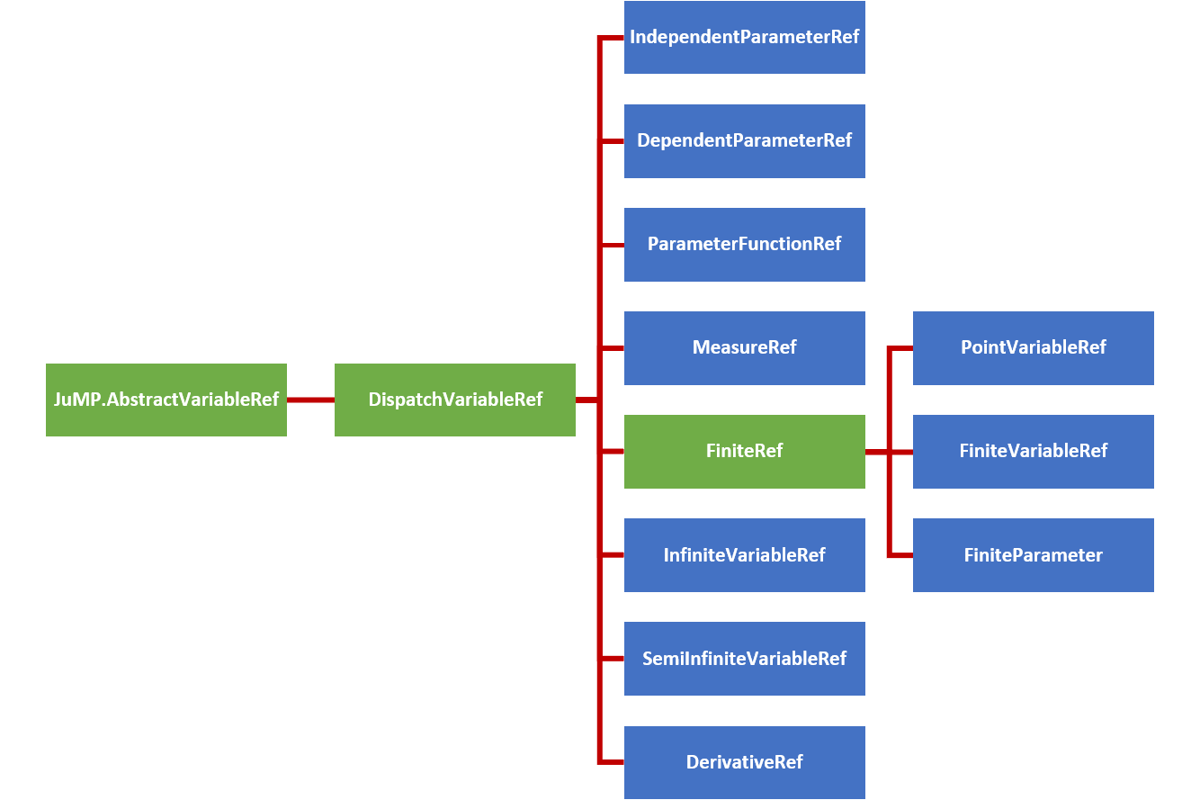
In consistently with JuMP expression support, GeneralVariableRef exists as a variable reference type that is able to represent any of the above concrete subtypes of DispatchVariableRef. This allows the expression containers to be homogeneous in variable type. This is a paradigm shift from previous versions of InfiniteOpt that used the hierarchy of types directly to construct expressions. This behavior led to stability and performance limitations and thus a has been discontinued.

However, the variable hierarchy is still used to create for variable methods. To accomplish this appropriate GeneralVariableRef dispatch methods are implemented (which are detailed in User Methods section at the bottom of this page) that utilize dispatch_variable_ref to create the appropriate concrete subtype of DispatchVariableRef and call the appropriate underlying method. These dispatch methods have been implemented for all public methods and the underlying methods are what are documented in the method manuals throughout the User Guide pages.

Affine Expressions

An affine expression pertains to a mathematical function of the form:

\[f_a(x) = a_1x_1 + ... + a_nx_n + b\]

where $x \in \mathbb{R}^n$ denote variables, $a \in \mathbb{R}^n$ denote coefficients, and $b \in \mathbb{R}$ denotes a constant value. Such expressions, are prevalent in any problem than involves linear constraints and/or objectives.

In InfiniteOpt, affine expressions can be defined directly using Julia's arithmetic operators (i.e., +, -, *, etc.) or using @expression. For example, let's define the expression $2y(t) + z - 3t$ noting that the following methods are equivalent:

julia> @infinite_parameter(model, t in [0, 10])
t

julia> @variable(model, y, Infinite(t))
y(t)

julia> @variable(model, z)
z

julia> expr = 2y + z - 3t
2 y(t) + z - 3 t

julia> expr = 2 * y + z - 3 * t
2 y(t) + z - 3 t

julia> expr = @expression(model, 2y + z - 3t)
2 y(t) + z - 3 t

julia> typeof(expr)
GenericAffExpr{Float64, GeneralVariableRef}

Notice that coefficients to variables can simply be put alongside variables without having to use the * operator. Also, note that all of these expressions are stored in a container referred to as a GenericAffExpr which is a JuMP object for storing affine expressions.

GenericAffExpr objects contain 2 fields which are:

• constant::CoefType The constant value of the affine expression.
• terms::OrderDict{VarType, CoefType} A dictionary mapping variables to coefficients.

For example, let's see what these fields look like in the above example:

julia> expr.terms
OrderedCollections.OrderedDict{GeneralVariableRef, Float64} with 3 entries:
  y(t) => 2.0
  z    => 1.0
  t    => -3.0

julia> expr.constant
0.0

Notice that the ordered dictionary preserves the order in which the variables appear in the expression.

More information can be found in the documentation for affine expressions in JuMP.

Quadratic Expressions

A quadratic function pertains to a mathematical function of the form:

\[f_q(x) = a_1x_1^2 + a_2 x_1 x_2 + ... + a_m x_n^2 + f_a(x)\]

where $x \in \mathbb{R}^n$ are the variables, $f_a(x): \mathbb{R}^n \mapsto \mathbb{R}$ is an affine function, and $m = n(n+1)/2$ is the number of unique combinations of variables $x$. Like affine expressions, quadratic expressions can be defined via Julia's arithmetic operators or via @expression. For example, let's define $2y^2(t) - zy(t) + 42t - 3$ using the following equivalent methods:

julia> expr = 2y^2 - z * y + 42t - 3
2 y(t)² - z*y(t) + 42 t - 3

julia> expr = @expression(model, 2y^2 - z * y + 42t - 3)
2 y(t)² - z*y(t) + 42 t - 3

julia> typeof(expr)
GenericQuadExpr{Float64, GeneralVariableRef}

Again, notice that coefficients need not employ *. Also, the object used to store the expression is a GenericQuadExpr which is a JuMP object used for storing quadratic expressions.

GenericQuadExpr object contains 2 data fields which are:

• aff::GenericAffExpr{CoefType,VarType} An affine expression
• terms::OrderedDict{UnorderedPair{VarType}, CoefType} A dictionary mapping quadratic variable pairs to coefficients.

Here the UnorderedPair type is unique to JuMP and contains the fields:

• a::AbstractVariableRef One variable in a quadratic pair
• b::AbstractVariableRef The other variable in a quadratic pair.

Thus, this form can be used to store arbitrary quadratic expressions. For example, let's look at what these fields look like in the above example:

julia> expr.aff
42 t - 3

julia> typeof(expr.aff)
GenericAffExpr{Float64, GeneralVariableRef}

julia> expr.terms
OrderedCollections.OrderedDict{UnorderedPair{GeneralVariableRef}, Float64} with 2 entries:
  UnorderedPair{GeneralVariableRef}(y(t), y(t)) => 2.0
  UnorderedPair{GeneralVariableRef}(z, y(t))    => -1.0

Notice again that the ordered dictionary preserves the order.

More information can be found in the documentation for quadratic expressions in JuMP.

Nonlinear Expressions

In this section, we walk you through the ins and out of working with general nonlinear (i.e., not affine or quadratic) expressions in InfiniteOpt.

Basic Usage

We can define nonlinear expressions in similar manner to how affine/quadratic expressions are made in JuMP. For instance, we can make an expression using normal Julia code outside a macro:

julia> @infinite_parameter(model, t ∈ [0, 1]); @variable(model, y, Infinite(t));

julia> expr = exp(y^2.3) * y - 42
(exp(y(t) ^ 2.3) * y(t)) - 42.0

julia> typeof(expr)
GenericNonlinearExpr{GeneralVariableRef}

Thus, the nonlinear expression expr of type GenericNonlinearExpr is created and can be readily incorporated into other expressions, the objective, and/or constraints. For macro-based definition, we simply use the @expression, @objective, and @constraint macros as normal:

julia> @expression(model, expr, exp(y^2.3) * y - 42)
(exp(y(t) ^ 2.3) * y(t)) - 42.0

julia> @objective(model, Min, ∫(0.3^cos(y^2), t))
∫{t ∈ [0, 1]}[0.3 ^ cos(y(t)²)]


julia> @constraint(model, constr, y^y * sin(y) + sum(y^i for i in 3:4) == 3)
constr : (((y(t) ^ y(t)) * sin(y(t))) + (y(t) ^ 3) + (y(t) ^ 4)) - 3.0 = 0, ∀ t ∈ [0, 1]

Natively, we support all the same nonlinear operators that JuMP does. See JuMP's documentation for more information.

We can interrogate which nonlinear operators our model currently supports by invoking all_nonlinear_operators. Moreover, we can add additional operators (see Adding Nonlinear Operators for more details).

Finally, we highlight that nonlinear expressions in InfiniteOpt support the same linear algebra operations as affine/quadratic expressions:

julia> @variable(model, v[1:2]); @variable(model, Q[1:2, 1:2]);

julia> @expression(model, v' * Q * v)
0.0 + ((Q[1,2]*v[1] + Q[2,2]*v[2]) * v[2]) + ((Q[1,1]*v[1] + Q[2,1]*v[2]) * v[1])

Function Tracing

In similar manner to Symbolics.jl, we support function tracing. This means that we can create nonlinear modeling expression using Julia functions that satisfy certain criteria. For instance:

julia> myfunc(x) = sin(x^3) / tan(2^x);

julia> expr = myfunc(y)
sin(y(t) ^ 3) / tan(2.0 ^ y(t))

However, there are certain limitations as to what internal code these functions can contain. The following CANNOT be used:

• loops (unless it only uses very simple operations)
• if-statements (see workaround below)
• unrecognized operators (if they cannot be traced).

We can readily work around the if-statement limitation using op_ifelse which is a nonlinear operator version of Base.ifelse and follows the same syntax. For example, the function:

function mylogicfunc(x)
    if x >= 0
        return x^3
    else
        return 0
    end
end

is not amendable for function tracing, but we can rewrite it as:

julia> function mylogicfunc(x)
          return op_ifelse(op_greater_than_or_equal_to(x, 0), x^3, 0)
       end
mylogicfunc (generic function with 1 method)

julia> mylogicfunc(y)
ifelse(y(t) >= 0, y(t) ^ 3, 0)

which is amendable for function tracing. Note that the basic logic operators (e.g., <=) have special nonlinear operator analogues when used outside of a macro. See JuMP's documentation for more details.

Linear Algebra

As described above in the Basic Usage Section, we support basic linear algebra operations with nonlinear expressions! This relies on our basic extensions of MutableArithmetics, but admittedly this implementation is not perfect in terms of efficiency.

julia> v' * Q * v # convenient linear algebra syntax
(+(0.0) + ((Q[1,1]*v[1] + Q[2,1]*v[2]) * v[1])) + ((Q[1,2]*v[1] + Q[2,2]*v[2]) * v[2])

julia> sum(v[i] * Q[i, j] * v[j] for i in 1:2, j in 1:2) # more efficient
((((v[1]*Q[1,1]) * v[1]) + ((v[2]*Q[2,1]) * v[1])) + ((v[1]*Q[1,2]) * v[2])) + ((v[2]*Q[2,2]) * v[2])

We can also set vectorized constraints using the .==, .<=, and .>= operators:

julia> @variable(model, W[1:2, 1:2]);

julia> @constraint(model, W * Q * v .== 0)
2-element Vector{InfOptConstraintRef}:
 ((+(0.0) + ((W[1,1]*Q[1,1] + W[1,2]*Q[2,1]) * v[1])) + ((W[1,1]*Q[1,2] + W[1,2]*Q[2,2]) * v[2])) - 0.0 = 0
 ((+(0.0) + ((W[2,1]*Q[1,1] + W[2,2]*Q[2,1]) * v[1])) + ((W[2,1]*Q[1,2] + W[2,2]*Q[2,2]) * v[2])) - 0.0 = 0

Adding Nonlinear Operators

In a similar spirit to JuMP and Symbolics, we can add nonlinear operators such that they can be directly incorporated into nonlinear expressions as atoms (they will not be traced). This is done via the @operator macro. We can register any operator that takes scalar arguments (which can accept inputs of type Real):

julia> h(a, b) = a * b^2; # an overly simple example operator

julia> @operator(model, op_h, 2, h);

julia> op_h(y, 42)
op_h(y(t), 42)

To highlight the difference between function tracing and operator definition consider the following example:

julia> f(a) = a^3;

julia> f(y) # user-function gets traced
y(t) ^ 3

julia> @operator(model, op_f, 1, f) # create nonlinear operator
NonlinearOperator(f, :op_f)

julia> op_f(y) # function is no longer traced
op_f(y(t))

Thus, nonlinear operators are incorporated directly. This means that their gradients and hessians will need to determined as well (typically occurs behind the scenes via auto-differentiation with the selected optimizer model backend). However, again please note that in this case tracing is preferred since f can be traced.

Let's consider a more realistic example where the function is not amenable to tracing:

julia> function g(a)
          v = 0
          for i in 1:4
              v *= v^a
              if v >= 1
                 return v
              end
          end
          return a
       end;

julia> @operator(model, op_g, 1, g);

julia> op_g(y)
op_g(y(t))

Notice this example is a little contrived still, highlighting that in most cases we can avoid adding operators. However, one exception to this trend, are functions from other packages that we might want to use. For example, perhaps we would like to use the eta function from SpecialFunctions.jl which is not natively supported:

julia> using SpecialFunctions

julia> @operator(model, op_eta, 1, eta)
NonlinearOperator(eta, :op_eta)

julia> op_eta(y)
op_eta(y(t))

Now in some cases we might wish to specify the gradient and hessian of a univariate operator to avoid the need for auto-differentiation. We can do this, simply by adding them as additional arguments in @operator:

julia> my_squared(a) = a^2; gradient(a) = 2 * a; hessian(a) = 2;

julia> @operator(model, op_square, 1, my_squared, gradient, hessian);

julia> op_square(y)
op_square(y(t))

Note the specification of the hessian is optional (it can separately be computed via auto-differentiation if need be).

For multivariate functions, we can specify the gradient following the same gradient function structure that JuMP uses:

julia> w(a, b) = a * b^2;

julia> function wg(v, a, b)
          v[1] = b^2
          v[2] = 2 * a * b
          return
       end;

julia> @operator(model, op_w, 2, w, wg)
NonlinearOperator(w, :op_w)

julia> op_w(42, y)
op_w(42, y(t))

Note that the first argument of the gradient needs to accept an AbstractVector{Real} that is then filled in place.

More Details

For more details, please consult JuMP's Documentation.